
A vehicle travels over a rough road. An aircraft completes a flight cycle. A machine runs through several operating speeds. A component experiences vibration that changes continuously with load, speed and operating condition.
Accelerometers can record all of it.
But recording the vibration is only the beginning.
The real engineering challenge is deciding which parts of that field data should be reproduced in the laboratory, how they should be represented, and whether the shaker can reproduce them without creating a test that is more—or less—severe than the real environment.
How do you turn field vibration data into a laboratory shaker test?
A practical field-to-laboratory workflow is:
Measure → Validate → Classify → Analyse → Build the target → Check shaker feasibility → Reproduce → Validate again
The process normally involves:
Measuring vibration at locations that represent the real input and critical structural response.
Recording enough operating conditions to describe the intended service environment.
Checking sensors, mounting, sampling and data quality before using the recordings.
Separating valid field events from measurement errors and non-representative conditions.
Analysing the data as time histories, PSDs, SRS or fatigue-related metrics according to the test objective.
Deciding whether to reproduce the original time waveform or develop a laboratory random vibration profile.
Checking the target against shaker force, velocity, displacement and acceleration limits.
Running the laboratory test under closed-loop control.
Comparing the controlled response with the intended field-derived target.
The important point is: Field data should not simply be copied into a vibration controller and called a test specification.
It needs engineering interpretation first.
Current aerospace test practice follows the same principle: actual flight data can be used when defining expected vibration environments, but the resulting verification criteria still require appropriate statistical treatment and test tailoring.
Field data is evidence - not automatically a test profile
Suppose an accelerometer records 40 minutes of vibration during a vehicle road test.
That file may contain:
Smooth-road driving
Rough-road sections
Braking
Cornering
Idling
High engine speed
Railway crossings or potholes
Driver stops
Sensor handling
One unusual impact
Several operating conditions that occur for very different lengths of time
If the complete 40-minute signal is repeated continuously on a shaker, the resulting laboratory test might have little relationship to the actual lifetime of the product. Likewise, selecting only the most severe 30 seconds could create a qualification test that dramatically over-represents rare events.
The first question is therefore not: “How do we replay this file?”
It is: “What does this file represent?”
The test engineer should understand:
What operating condition was recorded
How often that condition occurs in real service
How long it normally lasts
Whether the measured location represents the actual DUT input
Whether rare events are valid environmental events or measurement artefacts
Which failure mechanism the laboratory test is intended to reproduce
Only then can field measurement become a defensible test target.
The complete field-to-lab measurement chain

Road, machine, aircraft or operating condition

Measure vibration at representative locations

Record synchronized field data

Check clipping, dropouts, artefacts and operating conditions

Time history • PSD • SRS • Fatigue

TWR • Random PSD • Shock/SRS • Mixed profile

Closed-loop vibration control

Reproduce the selected environment

Apply the laboratory test

Compare laboratory response with field-derived target
A useful way to think about field-derived vibration testing is as one continuous measurement chain:
Real environment
↓
Sensor
↓
Field DAQ
↓
Validated time-history data
↓
Signal analysis
↓
Laboratory target
↓
Vibration controller
↓
Power amplifier
↓
Shaker
↓
Fixture and DUT
↓
Control and response accelerometers
Every stage can change the final result.
If the original sensor was poorly mounted, no amount of later signal processing can recover the true field vibration.
If the time history is valid but the PSD is generated from an unrepresentative operating period, the laboratory profile can still be wrong.
And if the field-derived target is correct but exceeds the shaker's displacement capability, the test cannot be reproduced simply by increasing controller drive.
A good field-to-lab programme therefore preserves measurement traceability from the original operating environment to the controlled laboratory response.
Step 1: Define the purpose before collecting field data
Before installing an accelerometer, define what the laboratory test must achieve.
Different objectives can require very different field measurements.
Durability testing
The objective may be to reproduce vibration that contributes to:
Fatigue cracking
Joint degradation
Connector failure
Fastener loosening
Material fatigue
Structural wear over service life
For durability work, the frequency, amplitude, number of cycles and duration of exposure all matter.
A short high-amplitude event and thousands of lower-amplitude cycles may contribute differently to damage.
Qualification testing
The objective may be to demonstrate that a component survives a defined operating environment with an appropriate engineering margin.
In this case, the field measurements may be used to establish or validate a qualification spectrum rather than reproduced literally.
Functional testing
Sometimes the question is not whether the product suffers permanent damage.
It is: Does it continue to operate correctly while experiencing real vibration?
Examples include:
Sensors
Electronic assemblies
Displays
Connectors
Relays
Optical systems
Control equipment
Preserving the timing characteristics of the environment may be particularly important for these tests.
Troubleshooting
Field data may also be collected because a product fails in service but passes the existing laboratory test.
The objective becomes finding what the laboratory test is missing.
For example:
A narrowband motor tone
A transient impact
A specific operating speed
An unusual resonance
A non-Gaussian peak distribution
Simultaneous environmental inputs
In this situation, examining the original time history may be more valuable than immediately reducing everything to an averaged PSD.
Step 2: Choose measurement locations that answer the engineering question
A field test can generate terabytes of perfectly accurate data from the wrong locations.
Sensor position should therefore follow the vibration transmission path.
A useful approach is to consider three types of measurement point.
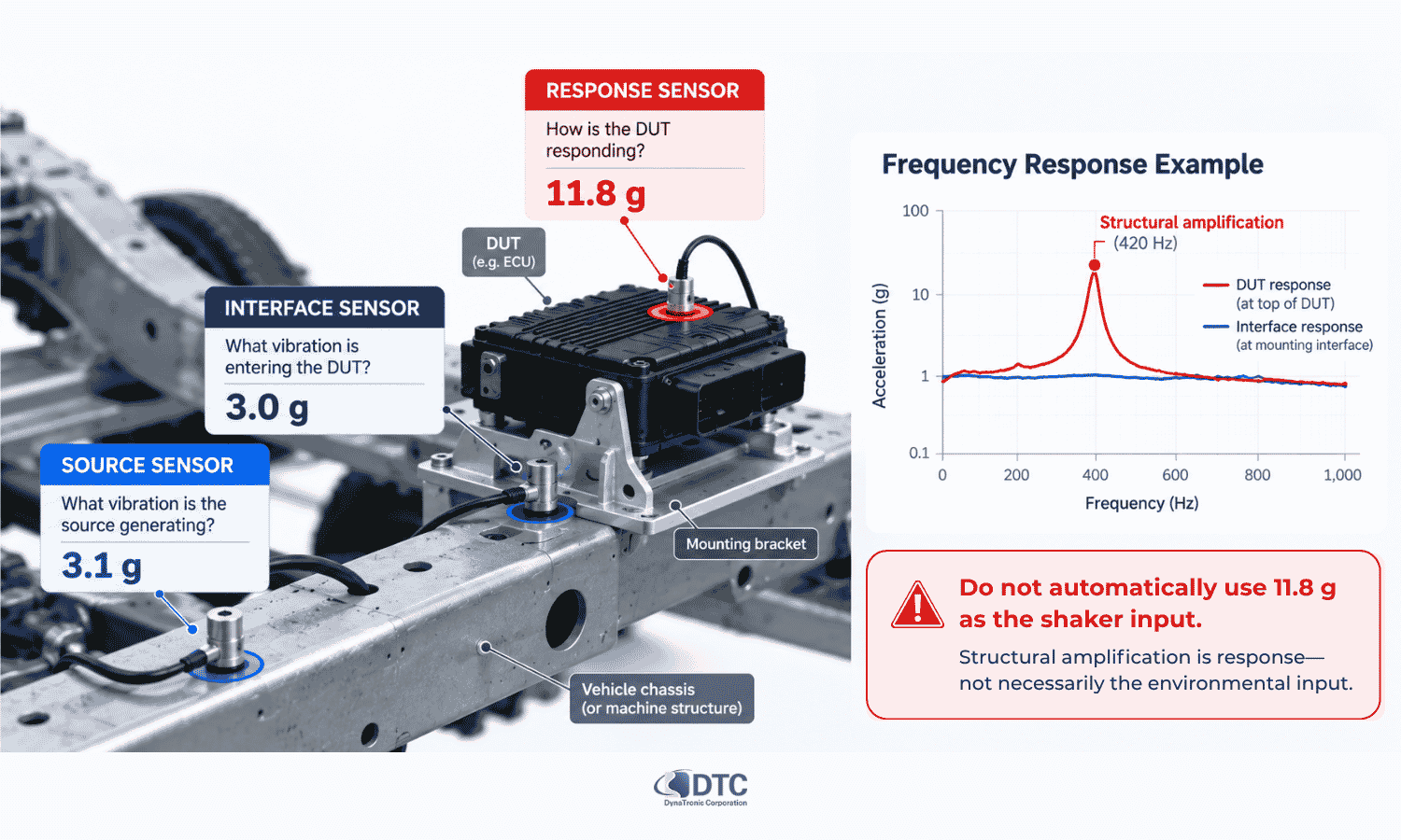
1. Source measurement
This tells you what the vibration source is generating.
Examples:
Vehicle chassis
Engine casing
Motor housing
Machine frame
Aircraft mounting structure
This can help characterise the source environment but may not represent what reaches the component.
2. Interface measurement
For developing a shaker test, this is often the most important measurement.
The accelerometer is positioned close to the mechanical interface through which vibration enters the DUT.
Examples include:
Component mounting bracket
Equipment mounting feet
Battery-pack mounting point
Electronic unit attachment interface
Seat rail
Structural attachment point
If the laboratory shaker is intended to reproduce the vibration entering the component, the target should generally be derived from a measurement that represents that boundary condition.
3. Response measurement
Additional sensors can be installed on the component itself.
They answer a different question: How does the DUT respond to the input?
Response measurements may identify:
Resonances
Local amplification
Flexible behaviour
Critical component motion
Structural mode participation
Do not automatically use a high internal response as the shaker control target.
If a resonance amplifies 3 g at the mounting interface into 12 g at an internal component, commanding the shaker to reproduce 12 g at the interface could substantially over-test the product.
A practical rule
Before placing every sensor, write down:
“I need this channel because…”
If there is no clear answer, reconsider whether the measurement is necessary.
Step 3: Select the correct accelerometer
The sensor must capture the vibration of interest without significantly changing it.
Important parameters include:
Sensitivity
Measurement range
Frequency response
Sensor mass
Noise floor
Environmental rating
Shock survivability
Output type
Cable configuration
DTC provides a range of IEPE, charge and vibration/shock accelerometers for different measurement levels and frequency ranges. Current DTC IEPE options include sensitivities intended for both relatively low-level vibration and considerably higher acceleration environments.
Sensitivity versus measurement range
A high-sensitivity accelerometer is useful for relatively low vibration levels because it produces a larger electrical output for the same acceleration. But high sensitivity usually comes with a lower maximum acceleration range.
A low-sensitivity accelerometer can measure higher acceleration without overload but may be less suitable when very small vibration signals must be resolved.
Select the sensor against the complete expected environment, not only the average value.
Allow for:
Resonance amplification
Road impacts
Start/stop events
Unexpected peaks
Structural response
Step 4: Treat sensor mounting as part of the measurement
The accelerometer does not measure vibration in isolation. It measures through its mounting interface.
A poor mounting method can introduce:
Additional resonance
High-frequency attenuation
Sensor movement
Cable-related noise
Incorrect axis orientation
Poor repeatability between tests
For demanding measurements, especially at higher frequencies, a rigid mounting method is generally preferable where the structure allows it.
Before recording, document:
Sensor model
Serial number
Sensitivity
Axis orientation
Exact location
Mounting method
Cable routing
Photographs of every sensor installation can be extremely valuable when data is reviewed weeks or months later.
This metadata should travel with the measurement file.
Step 5: Choose the sampling rate correctly
Sampling rate is one of the easiest field-measurement parameters to set incorrectly because “more samples” can sound automatically better. It is not that simple.
The sampling rate must be high enough to capture the required frequency range while working correctly with the acquisition system's anti-alias filtering.
According to NIST guidance on vibration-data acquisition, sampling must be at least twice the highest frequency component of interest to prevent aliasing, while higher ratios may be needed when accurate spectral amplitudes are required.
What is aliasing?
Imagine that vibration exists at a frequency higher than the measurement system can represent. If that high-frequency energy reaches the digital converter without adequate filtering, it can appear falsely at a lower frequency. The analysis may then show vibration that never existed at that apparent frequency. This is aliasing.
Once it has occurred during acquisition, it cannot simply be removed later by filtering the recorded file. That is why anti-alias filtering is part of the acquisition strategy—not a post-processing correction.
Nyquist is a limit, not necessarily a good design target
The theoretical Nyquist criterion says that the sampling rate must exceed twice the highest frequency being represented. But designing a field measurement at exactly that boundary leaves very little room for the real analogue filter transition band and practical spectral analysis.
Instead, define:
The highest physically meaningful frequency
The sensor's usable bandwidth
The DAQ anti-alias filter characteristics
The required frequency resolution
The required file length and storage
Then choose the sampling configuration.
DTC's portable VENZO 160 Dynamic Signal Data Acquisition and Analysis system provides simultaneous sampling up to 128 kHz in its portable 1–4 channel configuration with 24-bit analogue-to-digital conversion.
Step 6: Record representative operating conditions
One of the largest sources of error in field-derived test development is collecting too little context, rather than too little data.
Imagine measuring a vehicle for one hour without recording:
Speed
Road type
Payload
Tyre pressure
Driver behaviour
Vehicle operating mode
The acceleration file may be technically excellent but difficult to interpret. Instead, create an operating-condition matrix before measurement.
For a road vehicle, this could include:
| Condition | Example variables to record |
|---|---|
| Smooth road | Speed, payload, tyre condition |
| Rough road | Surface type, speed |
| Highway | Speed range, engine/motor state |
| Urban driving | Stops, acceleration, braking |
| Pothole/impact | Event location and speed |
| Cornering | Speed and turn severity |
| Idle | Engine or auxiliary equipment state |
For machinery, the equivalent matrix might use:
RPM
Load
Production state
Tool condition
Flow rate
Temperature
Start-up
Shutdown
For aerospace measurements it could include:
Taxi
Take-off
Climb
Cruise
Manoeuvre
Descent
Landing
NASA flight-vibration studies, for example, analyse measured acceleration separately for different flight conditions and manoeuvres because vibration spectra can change substantially with operating state.
Record metadata with the vibration signal
Useful metadata includes:
Date and time
DUT or vehicle configuration
Payload
Sensor configuration
Operating condition
Speed or RPM
Temperature
Event markers
Operator notes
Unusual occurrences
A time history without context is much harder to turn into a defensible laboratory specification.
Step 7: Do not clean the data before understanding the anomaly
Every real-world measurement contains unusual events. The mistake is assuming every unusual event is bad data.
When reviewing a field recording, classify questionable segments into three groups:
A. Valid and representative
These events genuinely occur and belong in the intended service environment.
Keep them.
B. Valid but non-representative
The measurement is real, but it may not belong in the test being developed.
For example:
A severe pothole encountered once during an otherwise normal durability route
An accidental impact during installation
A vehicle condition that the product rarely experiences
These segments should be analysed separately rather than silently mixed into an average.
C. Invalid measurement
Examples include:
Sensor cable hit
Loose accelerometer
Electrical dropout
Saturation
Clipping
Installation error
Data corruption
These should not influence the test target.
The useful question is not: “Does this point look like an outlier?”
It is: “What physically caused it?”
Deleting peaks merely because they are inconvenient can under-test the product.
Keeping measurement artefacts can over-test it.
Step 8: Check the time history before calculating anything else
Before generating a PSD, SRS or fatigue metric, inspect the raw time waveform.
Look for:
DC offset
Clipping
Sensor saturation
Dropouts
Unexpected spikes
Low-frequency drift
Changes in operating condition
Stationary versus non-stationary periods
Transient events
Changing RMS levels
Repeating patterns
Also calculate or review basic statistics such as:
Maximum
Minimum
Mean
RMS
Crest factor
Standard deviation
Kurtosis where relevant
This often reveals information that becomes less obvious after the data is converted into the frequency domain.
For example, two signals can produce similar PSDs while containing very different instantaneous peak behaviour.
Step 9: Decide what representation answers the test objective
There is no single correct way to convert field vibration into a laboratory target. The right representation depends on what the test needs to preserve.
Four particularly useful views are:
| Analysis | Best for answering |
|---|---|
| Time history | What actually happened and when? |
| PSD | How is random vibration energy distributed across frequency? |
| SRS | What transient structural response could a shock create? |
| Fatigue-related analysis | Which vibration environments may be more damaging over repeated exposure? |
These should not be treated as interchangeable.
Time-history analysis: preserve the sequence
A time history retains:
Amplitude
Timing
Transients
Changing RMS level
Event sequence
Non-stationary behaviour
Peak distribution
It can therefore be particularly important when the field environment contains:
Impacts
Start/stop events
Repeating cycles
Variable-speed operation
Non-Gaussian vibration
Strong amplitude modulation
Events where timing itself matters
If these characteristics are important to the product response, reducing the recording to one average PSD can remove useful information.
PSD analysis: understand broadband vibration energy
The power spectral density describes how random vibration energy is distributed with frequency.
A PSD is particularly useful when the environment can reasonably be represented as statistically stationary random vibration.
It can reveal:
Broadband energy
Dominant frequency regions
Narrowband peaks
Changes between operating conditions
Overall Grms
Resonant behaviour
For example, measured aircraft vibration has been analysed using PSDs to compare spectral levels and identify peaks associated with different flight conditions.
But remember: An averaged PSD does not preserve the original waveform.
It generally loses:
Exact timing
Phase sequence
Individual transient events
Event order
Some non-Gaussian characteristics
This is why converting field data into random vibration should be an engineering decision rather than an automatic processing step.
SRS analysis: identify transient severity
When the field environment contains short-duration impacts or shock-like events, a shock response spectrum can provide additional insight.
SRS estimates how a family of damped single-degree-of-freedom systems with different natural frequencies would respond to the measured transient.
It can help answer:
Which natural-frequency regions are strongly excited?
Are two impacts with different-looking time traces mechanically similar?
Is one rare transient driving the shock requirement?
Should that transient be tested separately from the random environment?
If shock events are significant, it may be inappropriate to blend them into one long PSD and assume the resulting random test reproduces the same structural response.
A separate shock or SRS requirement may be more defensible.
Fatigue-related analysis: distinguish energy from damage potential
For durability work, engineers may also need to understand whether different sections of a field record have different fatigue-damage potential.
Two environments with similar RMS acceleration do not necessarily produce identical fatigue effects.
Important variables can include:
Frequency
Cycle count
Resonance
Duration
Material S–N behaviour
Damping
Peak distribution
A Fatigue Damage Spectrum, for example, is used to compare the damage potential of vibration loading across a range of hypothetical structural natural frequencies. Recent research continues to use FDS-based methods for synthesising accelerated durability tests from real mission data, while also examining their assumptions and limitations.
FDS should not be treated as a direct prediction of the exact fatigue life of every real component.
It is better considered one tool for comparing and shaping test severity, together with structural knowledge and the actual failure mechanism.
Step 10: Choose between time waveform replication and random vibration testing
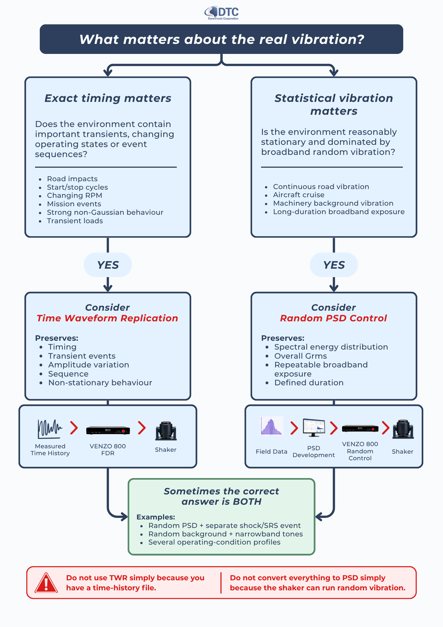
This is one of the most important decisions in the field-to-lab process.
Use time waveform replication when the original sequence matters
Time waveform replication—often abbreviated TWR or described as field data replication—uses measured field data as the target for closed-loop shaker reproduction.
It can be appropriate when:
The environment is strongly non-stationary
Transients are important
The load changes with time
A specific road or mission event must be reproduced
Peaks and timing should be retained
A repeating operational sequence must be recreated
Converting to a stationary PSD would remove important behaviour
DTC's VENZO 800 vibration controller includes Field Data Replication functionality for importing measured vibration data such as acceleration and reproducing it through the shaker control system.
Use a random PSD test when the statistical environment matters more than the exact sequence
A derived random profile may be more suitable when:
The measured process is reasonably stationary
Long service exposure must be condensed
Repeatability between laboratory tests is important
The qualification standard expects a PSD
Broadband vibration dominates
Exact event sequence is not important to the failure mechanism
The laboratory can then run closed-loop random control against the derived PSD.
VENZO 800 supports real-time closed-loop control of random PSD profiles.
TWR versus random testing: a practical comparison
| Question | Time waveform replication | Derived random PSD |
|---|---|---|
| Preserves event timing? | Yes | No |
| Preserves specific transients? | Yes | Generally not directly |
| Reproduces exact field sequence? | Intended to approximate it under closed-loop control | No |
| Easy to accelerate? | More difficult | Often easier |
| Suitable for stationary broadband environment? | Possible | Often appropriate |
| Suitable for strongly non-stationary data? | Often | May lose important behaviour |
| Repeatability | High with controlled reproduction | High |
| Test definition | Time history | PSD + duration |
| Main risk | Reproducing irrelevant/invalid field content | Removing important temporal or peak characteristics |
Neither method is inherently superior. The test method should preserve the characteristics connected to the engineering objective.
Step 11: Do not automatically envelope every PSD peak
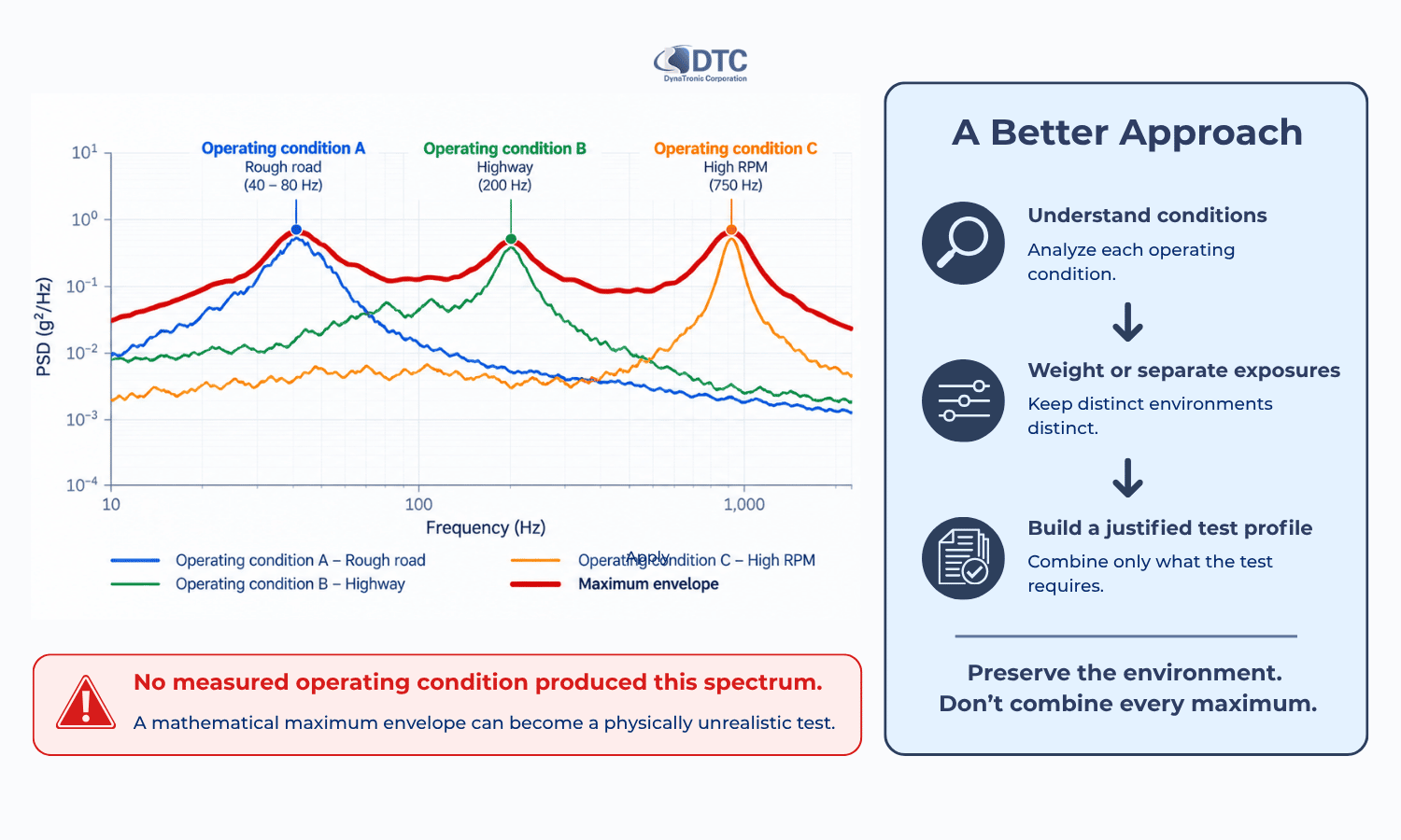
Suppose you calculate PSDs for 30 different operating segments. A simple approach would be to take the highest PSD value at every frequency and connect those maximum values into one envelope. It looks conservative. But consider what that curve means.
The peak at 40 Hz may have occurred during one operating condition.
The peak at 200 Hz may have occurred during another.
The peak at 800 Hz may have occurred only once.
No actual operating condition may ever produce all three simultaneously.
If you reproduce the envelope continuously, the DUT can be subjected to an environment that never existed.
This is one mechanism by which a field-derived test becomes over-testing.
NASA vibration-test guidance similarly states that the frequency range of a test PSD should correspond to the range of significant amplitudes in the source environment, and recognises that test specifications need to account for facility and hardware realities rather than simply reproducing every measured feature indiscriminately.
Better approaches may include:
Separating operating conditions
Weighting them by service duration
Defining several test stages
Preserving meaningful narrowband components separately
Using statistical qualification levels
Evaluating fatigue equivalence
Creating a justified envelope rather than a mathematical maximum of everything
The choice depends on the programme.
Step 12: Define duration as carefully as amplitude
A shaker test profile without a meaningful duration is incomplete.
Imagine that the field measurement represents:
10 minutes of rough road
experienced once every 20 operating hours
over a 5,000-hour intended service life
A durability test may need to account for the accumulated exposure.
But simply multiplying the amplitude to make the test shorter can change the failure physics.
Acceleration, frequency and cycles interact with:
Stress
Resonance
Material fatigue
Joint behaviour
Nonlinearities
Thermal effects
Accelerated test development therefore requires more than increasing Grms until the desired test time fits the laboratory schedule.
Any acceleration factor should be supported by an appropriate fatigue or structural model and validated against the intended failure mechanism.
Step 13: Check whether the shaker can physically reproduce the target
A mathematically valid field-derived target may still be impossible to reproduce on the available shaker.
Four limits should always be checked.
Acceleration
Can the shaker generate the required acceleration with the combined moving mass?
That mass includes more than the DUT:
Armature
Fixture
Head expander where applicable
DUT
Cables and auxiliary components
Force
Required force depends on the moving mass and dynamic behaviour of the complete system.
Structural resonances can change the demand significantly.
Velocity
A profile can remain within the acceleration capability while exceeding the shaker's velocity limit.
This is particularly relevant at lower and intermediate frequencies.
Displacement
Low-frequency vibration can require large armature travel.
A field waveform containing slow, large-amplitude motion may exceed the available displacement even when its peak acceleration appears modest.
That is why “the field accelerometer recorded it” does not automatically mean “the electrodynamic shaker can reproduce it.”
Before testing, calculate or review the target against the shaker's:
Force + acceleration + velocity + displacement envelope.
Step 14: Check whether low-frequency content is meaningful
Field measurements can contain low-frequency components caused by:
Vehicle body movement
Suspension travel
Orientation change
Sensor tilt
Structural motion
Drift
Environmental effects
Some of this information may be physically important. Some may be outside the intended shaker-test objective. And some may demand more displacement than an electrodynamic shaker can generate. Do not simply high-pass the data until the displacement calculation becomes convenient.
Instead ask:
Is the low-frequency motion part of the relevant damage mechanism?
Does it represent rigid-body motion rather than component vibration?
Is it an acquisition artefact?
Should another type of actuator reproduce it?
Can the test objective justify removing it?
Every significant edit to field data should have an engineering reason.
Step 15: Prepare the waveform or target without destroying what matters
Depending on the test method, preprocessing may include:
Removing a justified DC offset
Cropping invalid segments
Separating operating states
Applying appropriate filtering
Resampling correctly
Converting engineering units
Combining representative segments
Applying documented scaling
Constructing a PSD
Defining test duration
Preparing an SRS or separate shock requirement
Keep the original raw data unchanged. Never make the edited file the only surviving copy.
A useful data hierarchy is:
RAW → VALIDATED → PROCESSED → TEST TARGET
This creates traceability.
If someone later asks why a 600 Hz peak disappeared from the laboratory specification, the engineering team should be able to reconstruct the decision.
Step 16: Establish a low-level laboratory control test first
Do not begin with the full field-derived test level. Start at a reduced level.
This allows the engineering team to examine:
Shaker response
Fixture behaviour
Control stability
Resonances
Drive demand
Response-channel amplification
Sensor integrity
Force, velocity and displacement margins
The shaker, fixture and DUT form a new dynamic system.
That laboratory system is not identical to the field installation.
A resonance in the fixture can change the response even if the target waveform itself is correct.
Use the low-level run to understand those differences before progressing toward the full target.
Step 17: Validate the reproduced laboratory environment
Pressing “Run” does not complete field data replication.
Validation should ask: Did the DUT receive the environment we intended to reproduce?
Compare the laboratory control and response measurements with the field-derived target.
Depending on the test method, evaluate:
Time domain
Waveform shape
RMS
Peaks
Transients
Timing
Statistical distribution
Frequency domain
PSD
Narrowband features
Resonances
Spectral deviations
Shock response
SRS where relevant
Structural response
Response accelerometers
Critical component motion
Resonance changes
Limiting channels
Test-system behaviour
Drive level
Shaker limits
Fixture response
Control error
The objective is not merely for the controller screen to look close to the target.
The objective is for the test article to experience the intended laboratory environment without introducing unacceptable test-system artefacts.
Avoiding over-testing
A field-derived test can become more severe than reality when engineers:
Use only the most severe recorded event
Envelope unrelated operating conditions
Repeat rare transients too frequently
Increase amplitude without considering fatigue physics
Control to a structural response instead of the input interface
Include measurement artefacts
Ignore real service duty cycle
Extend the test duration unnecessarily
Add excessive qualification margin on top of an already conservative envelope
Over-testing can cause failures that the product would not experience in normal service.
It can also drive unnecessary redesign.
A conservative test is not automatically a better test.
A good test is one whose severity can be technically justified.
Avoiding under-testing
Under-testing can occur when engineers:
Record too few operating conditions
Remove legitimate high-amplitude events
Average away narrowband peaks
Ignore transient shocks
Select an unrepresentative sensor location
Clip the field measurement
Use inadequate sampling bandwidth
Ignore high-response service conditions
Reproduce only an average operating state
Fail to account for total service duration
An easy-to-pass test is no more useful than an unrealistically severe one.
The objective is environmental equivalence—not simply achieving a pass.
A useful three-question test before approving the laboratory profile
Before finalising any field-derived test, ask three questions.
1. Is it representative?
Can each important part of the profile be traced back to a real operating condition or justified engineering requirement?
2. Is it mechanically meaningful?
Does the profile preserve the aspects of the environment associated with the expected response or failure mechanism?
3. Is it physically reproducible?
Can the shaker, amplifier, fixture and controller reproduce it safely within their operating limits?
If the answer to any of these questions is no, the profile is not ready.
Recommended DTC workflow: sensor → VENZO 160 → VENZO 800
DTC can support the complete field-to-laboratory workflow rather than only the final shaker-control stage.
1. Capture the environment with appropriate sensors
Select accelerometers according to:
Expected level
Frequency range
Measurement location
Environmental conditions
Sensor mass
Output type
Review DTC's vibration and shock sensor range when defining the field measurement chain.
2. Record and analyse field vibration with VENZO 160
VENZO 160 Dynamic Signal Data Acquisition & Analysis supports spectrum analysis and time-domain counting functions in addition to dynamic measurement capabilities. The portable configuration provides 1–4 inputs, simultaneous sampling up to 128 kHz and 24-bit conversion, while DTC describes the wider system architecture as expandable as measurement requirements increase.
This stage can be used to examine the measured environment before a test target is created.
3. Reproduce the selected environment with VENZO 800
VENZO 800 Series Vibration Controller supports:
Field Data Replication
Random vibration control
Sine vibration
Classical shock
For field data replication, measured vibration data such as acceleration can be imported for laboratory reproduction. VENZO 800 configurations provide sampling rates up to 204.8 kHz and are available with different input-channel capacities depending on the model.
The correct VENZO configuration should be selected according to:
Number of control channels
Monitoring and limiting channels
Shaker configuration
Required test type
Field-data bandwidth
Future expansion
DTC's current controller and DAQ datasheets are also available from the DTC technical download centre.
Example: turning a road measurement into a laboratory test
Consider an electronic module mounted to a commercial vehicle. Engineers want to reproduce its service vibration in the laboratory.
Field stage
A triaxial accelerometer is installed near the module's mounting interface. Additional response accelerometers are installed on the module housing.
The vehicle is measured during:
Urban driving
Highway driving
Smooth road
Rough road
Braking
Several known severe road sections
Vehicle speed and road condition are logged alongside the vibration recording.
Validation stage
Engineers identify:
One cable-impact artefact
Several genuine pothole events
Different vibration levels between road types
A persistent narrowband component associated with vehicle operation
One strong resonance in the module response that is not present at the mounting interface
The cable-impact event is removed as invalid.
The module resonance is retained as response information—but is not used directly as the shaker input.
Analysis stage
The team calculates:
Time histories
PSDs for individual road conditions
Overall RMS levels
Peak statistics
Shock response for the severe impact events
Exposure duration for each road type
Test-definition stage
They decide that normal road vibration is sufficiently stationary to represent with several PSD stages.
The rare pothole events are treated separately rather than increasing the broadband PSD to cover them continuously.
The narrowband operating component is reviewed to determine whether it needs separate reproduction.
Laboratory stage
A reduced-level random test is run first.
The fixture is checked for resonances.
The final random profiles are then controlled using the mounting-interface accelerometer while response sensors monitor the DUT.
The laboratory responses are compared with the field measurements.
This test has now been derived from field data.
It is not merely a field recording played through a shaker.
That distinction is the difference between data replay and environmental test engineering.
Common questions about field data replication
-
Technically, a measured time history can be used as the basis for field data or time waveform replication.
However, the recording should first be checked for sensor errors, bandwidth, offsets, invalid events, appropriate measurement location and shaker feasibility.
The complete raw recording is not automatically a valid test profile.
-
The terms are commonly used for closely related processes in which a measured or defined time waveform is reproduced under closed-loop laboratory control.
DTC uses the term Field Data Replication (FDR) for this capability in the VENZO 800 vibration-control platform.
-
Only when a random PSD is a suitable representation of the environment and test objective.
A PSD can be effective for stationary broadband vibration but does not preserve the exact event sequence or all transient and non-Gaussian characteristics of the original time history.
-
No.
Every important peak should be understood, but not every peak automatically belongs in the final test.
Determine whether it is:
A representative environmental event
A valid but rare condition
A separate shock requirement
A structural response
A measurement artefact
Then decide how it should be treated.
-
There is no universal duration.
The recording must be long enough to represent the relevant operating conditions and provide reliable statistical information for the intended analysis.
NIST notes that spectral estimates from finite records contain statistical uncertainty and that averaging multiple stationary data segments improves the reliability of spectral estimates.
-
Choose the sampling rate from the highest frequency that matters to the test, the sensor bandwidth and the DAQ's anti-alias filtering.
Sampling at just twice the target bandwidth represents the theoretical lower bound rather than an automatically optimal practical setting.
-
No.
Grms represents overall RMS acceleration, but test severity also depends on how the energy is distributed across frequency, exposure duration, structural resonances, peak statistics and the failure mechanism.
-
Potentially, but reducing months or years of service exposure to a short laboratory test requires engineering justification.
Increasing amplitude can change structural response and failure mechanisms. Fatigue-equivalent approaches may help, but their assumptions and limitations should be understood before applying acceleration factors.
-
Yes. DTC lists Field Data Replication as one of the core VENZO 800 vibration-control modes, using imported measured vibration information such as acceleration as the replication target.
-
Not every application does, but separating the field-measurement and laboratory-control stages can be useful.
A portable DAQ such as VENZO 160 can capture and analyse the real environment, while VENZO 800 provides closed-loop laboratory shaker control.
The appropriate configuration depends on channel count, sensors, required analysis and test workflow.
From measured vibration to a defensible laboratory test
The purpose of field data collection is not simply to produce a large acceleration file. It is to understand the environment well enough to reproduce the parts that matter.
A reliable workflow should preserve the connection between:
Where the vibration was measured → what operating condition produced it → how the data was processed → why the laboratory target was created → what the DUT actually experienced on the shaker.
That traceability helps prevent two costly mistakes:
Over-testing a product against an environment it will never experience.
and
Under-testing it because important field behaviour disappeared during data reduction.
The right laboratory target may be:
The original time waveform
A processed time waveform
One or several random PSD profiles
A shock or SRS requirement
A mixed test sequence
A fatigue-equivalent durability profile
There is no single conversion that is correct for every field measurement.
The right answer depends on the physical environment, the DUT, the expected failure mechanism and the purpose of the test.
Have field vibration data but are not sure how to turn it into a shaker test?
Send DTC:
A sample time-history file
Measurement units and sampling rate
Sensor locations
Operating-condition information
DUT and fixture details
Shaker and amplifier models, if already available
The objective of the laboratory test
DTC can help review the measurement and determine the appropriate sensor, VENZO 160 DAQ, analysis and VENZO 800 vibration-control workflow.